Numerical
Solution of the Heat Equation
In this section we will use MATLAB to
numerically solve the heat equation
(also known as the diffusion equation),
a partial differential equation that describes many physical processes
including conductive heat flow or the diffusion of an impurity in a motionless
fluid. You can picture the process of
diffusion as a drop of dye spreading in a glass of water. (To a certain extent you could also picture
cream in a cup of coffee, but in that case the mixing is generally complicated
by the fluid motion caused by pouring the cream into the coffee, and is further
accelerated by stirring the coffee.)
The dye consists of a large number of individual particles, each of
which repeatedly bounces off of the surrounding water molecules, following an
essentially random path. There are so
many dye particles that their individual random motions form an essentially
deterministic overall pattern as the dye spreads evenly in all directions (we ignore
here the possible effect of gravity).
In a similar way, you can imagine heat energy spreading through random
interactions of nearby particles.
In a three-dimensional medium, the heat
equation is
 .
.
Here u
is a function of t, x, y,
and z that represents the
temperature, or concentration of impurity in the case of diffusion, at time t at position (x, y, z) in the medium. The constant k depends on the materials involved, and is called the thermal conductivity in the case of heat
flow, and the diffusion coefficient
in the case of diffusion. To simplify
matters, let us assume that the medium is instead one-dimensional. This could represent diffusion in a thin
water-filled tube or heat flow in a thin insulated wire; let us think primarily
of the case of heat flow. Then the
partial differential equation becomes
![]()
where u(x, t)
is the temperature at time t a
distance x along the wire.
A
Finite-Difference Solution
To solve this partial differential equation
we need both initial conditions of
the form u(x, 0) = f(x), where f(x) gives the
temperature distribution in the wire at time 0, and boundary conditions at the endpoints of the wire, call them x = a
and x = b. We choose so-called
Dirichlet boundary conditions u(a, t)
= ![]() and u(b,
t) =
and u(b,
t) = ![]() , which correspond to the temperature being held steady at
values
, which correspond to the temperature being held steady at
values ![]() and
and ![]() at the two
endpoints. Though an exact solution is
available in this scenario, let us instead illustrate the numerical method of finite differences.
at the two
endpoints. Though an exact solution is
available in this scenario, let us instead illustrate the numerical method of finite differences.
To begin with, on the computer we can only
keep track of the temperature u at a
discrete set of times and a discrete set of positions x. Let the times be 0, Dt,
2Dt, …, NDt,
and let the positions be a, a + Dx, …, a + JDx =
b, and let ![]() = u(a
+ jDt, nDt). Rewriting the partial differential equation in terms of finite
difference approximations to the derivatives, we get
= u(a
+ jDt, nDt). Rewriting the partial differential equation in terms of finite
difference approximations to the derivatives, we get
![]() .
.
(These are the simplest approximations we can
use for the derivatives, and this method can be refined by using more accurate
approximations, especially for the t
derivative.) Thus if for a particular n, we know the values of ![]() for all j, we can solve the equation above to
find
for all j, we can solve the equation above to
find ![]() for each j:
for each j:
![]()
where s
= kDt/(Dx)2. In other words, this equation tells us how
to find the temperature distribution at time step n+1 given the temperature distribution at time step n.
(At the endpoints j = 0 and j = J,
this equation refers to temperatures outside the prescribed range for x, but at these points we will ignore
the equation above and apply the boundary conditions instead.) We can interpret this equation as saying
that the temperature at a given location at the next time step is a weighted
average of its temperature and the temperatures of its neighbors at the current
time step. In other words, in time Dt, a given section of the
wire of length Dx
transfers to each of its neighbors a portion s of its heat energy and keeps the remaining portion 1-2s
of its heat energy. Thus our numerical
implementation of the heat equation is a discretized version of the microscopic
description of diffusion we gave initially, that heat energy spreads due to
random interactions between nearby particles.
The following M-file, which we have named heat.m, iterates the procedure
described above.
function u = heat(k, x, t, init,
bdry)
% solve the 1D heat equation on
the rectangle described by
% vectors x and t with u(x, t(1))
= init and Dirichlet boundary
% conditions u(x(1), t) = bdry(1),
u(x(end), t) = bdry(2).
J = length(x);
N = length(t);
dx = mean(diff(x));
dt = mean(diff(t));
s = k*dt/dx^2;
u = zeros(N,J);
u(1, :) = init;
for n = 1:N-1
u(n+1,
2:J-1) = s*(u(n, 3:J) + u(n, 1:J-2)) + (1 - 2*s)*u(n, 2:J-1);
u(n+1,
1) = bdry(1);
u(n+1,
J) = bdry(2);
end
The function heat takes as inputs the value of k,
vectors of t and x values, a vector init of initial values (which is
assumed to have the same length as x), and a vector bdry containing a pair of boundary values.
Its output is a matrix of u
values. Notice that since indices of
arrays in MATLAB must start at 1, not 0, we have deviated slightly from our
earlier notation by letting n=1 represent the initial time
and j=1 represent the left
endpoint. Notice also that in the first
line following the for statement, we compute an
entire row of u, except for the first and
last values, in one line; each term is a vector of length J-2, with the index j increased by 1 in the term u(n,3:J) and decreased by 1 in the
term u(n,1:J-2).
Let's use the M-file above to solve the
one-dimensional heat equation with k
= 2 on the interval -5 £ x £ 5 from time 0 to time 4,
using boundary temperatures 15 and 25, and initial temperature distribution of
15 for x < 0 and 25 for x > 0. You can imagine that two separate wires of
length 5 with different temperatures are joined at time 0 at position x = 0, and each of their far ends
remains in an environment that holds it at its initial temperature. We must choose values for Dt and Dx; let's try Dt = 0.1 and Dx = 0.5, so that there are 41
values of t ranging from 0 to 4 and
21 values of x ranging from -5 to 5.
xvals = linspace(-5, 5,
21);
init = 20 + 5*sign(xvals);
uvals = heat(2, tvals,
xvals, init, [15 25]);
surf(xvals, tvals, uvals)
xlabel x; ylabel t; zlabel u
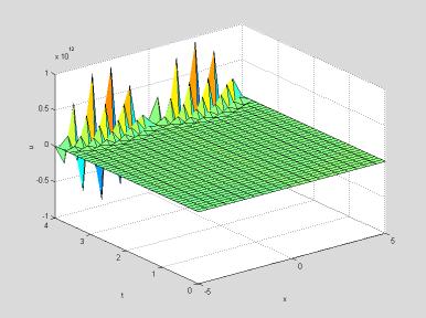
Here
we used surf to show the entire solution
u(x,
t).
The output is clearly unrealistic; notice the scale on the u axis!
The numerical solution of partial differential equations is fraught with
dangers, and instability like that seen above is a common problem with finite
difference schemes. For many partial
differential equations a finite difference scheme will not work at all, but for
the heat equation and similar equations it will work well with proper choice of
Dt and Dx. One might be inclined to think that since our choice of Dx was larger, it should be
reduced, but in fact this would only make matters worse. Ultimately the only parameter in the
iteration we're using is the constant s,
and one drawback of doing all the computations in an M-file as we did above is
that we do not automatically see the intermediate quantities it computes. In this case we can easily calculate that s = 2(0.1)/(0.5)2 = 0.8. Notice that this implies that the
coefficient 1-2s of ![]() in the iteration
above is negative. Thus the
"weighted average" we described before in our interpretation of the
iterative step is not a true average; each section of wire is transferring more
energy than it has at each time step!
in the iteration
above is negative. Thus the
"weighted average" we described before in our interpretation of the
iterative step is not a true average; each section of wire is transferring more
energy than it has at each time step!
The
solution to the problem above is thus to reduce the time step Dt; for instance, if we cut it
in half, then s = 0.4, and all
coefficients in the iteration are positive.
uvals = heat(2, tvals, xvals, init, [15 25]);
surf(xvals, tvals, uvals)
xlabel x; ylabel t; zlabel u
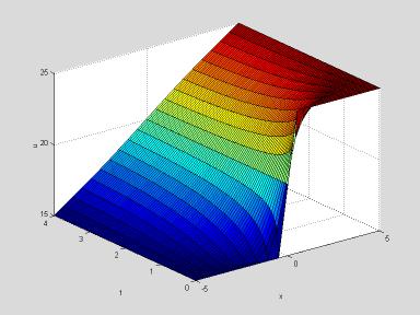
This
looks much better! As time increases,
the temperature distribution seems to approach a linear function of x.
Indeed u(x, t) = 20 + x is the limiting "steady
state" for this problem; it satisfies the boundary conditions and it
yields 0 on both sides of the partial differential equation.
Generally
speaking, it is best to understand some of the theory of partial differential
equations before attempting a numerical solution like we have done here. However for this particular case at least,
the simple rule of thumb of keeping the coefficients of the iteration positive
yields realistic results. A theoretical
examination of the stability of this finite difference scheme for the
one-dimensional heat equation shows that indeed any value of s between 0 and 0.5 will work, and
suggests that the best value of Dt
to use for a given Dx
is the one that makes s = 0.25[1]. Notice that while we can get more accurate
results in this case by reducing Dx,
if we reduce it by a factor of 10 we must reduce Dt
by a factor of 100 to compensate, making the computation take 1000 times as
long and use 1000 times the memory!
The Case of
Variable Conductivity
Earlier
we mentioned that the problem we solved numerically could also be solved
analytically. The value of the
numerical method is that it can be applied to similar partial differential
equations for which an exact solution is not possible or at least not known. For example, consider the one-dimensional
heat equation with a variable coefficient,
representing an inhomogeneous material with varying thermal conductivity k(x),
 .
.
For
the first derivatives on the right-hand side, we use a symmetric finite
difference approximation, so that our discrete approximation to the partial
differential equations becomes
![]() ,
,
where
![]() = k(a
+ jDx). Then the time iteration for this method is
= k(a
+ jDx). Then the time iteration for this method is
![]() ,
,
where
![]() =
= ![]() Dt/(Dx)2. In the following M-file, which we called heatvc.m, we modify our previous
M-file to incorporate this iteration.
Dt/(Dx)2. In the following M-file, which we called heatvc.m, we modify our previous
M-file to incorporate this iteration.
function u =
heatvc(k, x, t, init, bdry)
% solve the 1D
heat equation with variable coefficient k on the rectangle
% described by
vectors x and t with u(x, t(1)) = init and Dirichlet boundary
% conditions
u(x(1), t) = bdry(1), u(x(end), t) = bdry(2).
J = length(x);
N = length(t);
dx =
mean(diff(x));
dt =
mean(diff(t));
s = k*dt/dx^2;
u = zeros(N,J);
u(1,:) = init;
for n = 1:N-1
u(n+1, 2:J-1) = s(2:J-1).*(u(n, 3:J) + u(n,
1:J-2)) + ...
(1 - 2*s(2:J-1)).*u(n,2:J-1) + ...
0.25*(s(3:J) - s(1:J-2)).*(u(n, 3:J) - u(n,
1:J-2));
u(n+1, 1) = bdry(1);
u(n+1, J) = bdry(2);
end
Notice
that k is now assumed to be a
vector with the same length as x, and that as a result so is
s. This in turn requires that we use vectorized multiplication in
the main iteration, which we have now split into three lines.
Let's
use this M-file to solve the one-dimensional variable coefficient heat equation
with the same boundary and initial conditions as before, using k(x)
= 1 + ![]() . Since the maximum
value of k is 2, we can use the same
values of Dt and Dx
as before.
. Since the maximum
value of k is 2, we can use the same
values of Dt and Dx
as before.
uvals = heatvc(kvals, tvals, xvals, init, [15 25]);
surf(xvals, tvals, uvals)
xlabel x; ylabel t; zlabel u
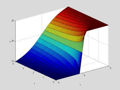
In
this case the limiting temperature distribution is not linear; it has a steeper
temperature gradient in the middle, where the thermal conductivity is
lower. Again one could find the exact
form of this limiting distribution, u(x, t)
= 20(1 + (1/p)arctan(x/5)), by setting the t
derivative to zero in the original equation and solving the resulting ordinary
differential equation.
You
can use the method of finite differences to solve the heat equation in two or three
space dimensions as well. For this and
other partial differential equations with time and two space dimensions, you
can also use the PDE Toolbox, which implements the more sophisticated finite element method.
A SIMULINK Solution
We can also solve the heat equation using
SIMULINK. To do this we continue to
approximate the x-derivatives with
finite differences, but think of the equation as a vector-valued ordinary
differential equation, with t as the
independent variable. SIMULINK solves
the model using MATLAB's ODE solver, ode45. To illustrate how to do this,
let's take the same example we started with, the case where k = 2 on the interval -5
£ x £ 5 from time 0 to time 4,
using boundary temperatures 15 and 25, and initial temperature distribution of
15 for x < 0 and 25 for x > 0. We replace u(x,t) for fixed t by the
vector u
of values of u(x,t), with, say, x = -5:5. Here there are 11 values of x
at which we are sampling u, but since
u(x,t) is pre-determined at the endpoints,
we can take u to be a 9-dimensional vector, and we just tack on the values at the
endpoints when we're done. Since we're
replacing ![]() by its finite difference approximation and we've taken Dx =
1 for simplicity, our equation becomes the vector-valued ODE
by its finite difference approximation and we've taken Dx =
1 for simplicity, our equation becomes the vector-valued ODE
![]() .
.
Here the right-hand side represents our
approximation to k![]() . The matrix A is:
. The matrix A is:
 , since we are replacing
 ![]() at (n, t)
with u(n-1,t) - 2u(n,t) + u(n+1, t). We represent this matrix in MATLAB's
notation by:
at (n, t)
with u(n-1,t) - 2u(n,t) + u(n+1, t). We represent this matrix in MATLAB's
notation by:
-2*eye(9) +
[zeros(8,1),eye(8);zeros(1,9)] + [zeros(8,1),eye(8);zeros(1,9)]'
The vector c comes from the boundary
conditions, and has 15 in its first entry, 25 in its last entry, and 0's in
between. We represent it in MATLAB's notation as [15;zeros(7,1);25]. The
formula for c comes from the fact that u(1) represents u(-4,t), and ![]() at this point is approximated by
at this point is approximated by
u(-5,t)
- 2u(-4,t)
+ u(-3, t) = -15 -2 u(1) + u(2),
and similarly at the other endpoint. Here's a SIMULINK model representing this equation:
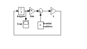
Note that one needs to specify the initial
conditions for u as Block Parameters for the Integrator block, and that in the
Block Parameters dialog box for the Gain block, one needs to set the multiplication
type to "Matrix". Since u(1) through u(4) represent u(x,
t) at x = -4 through -1, and u(6) through u(9) represent u(x,
t) at x = 1 through 4, we take the initial value of u to be [15*ones(4,1);20;25*ones(4,1)]. (20 is a compromise at x
= 0, since this is right in the middle of the regions where u is 15 and 25.) The output from the model is displayed in
the Scope block in the form of graphs of the various entries of u as function of t, but it's more useful to save the output to the MATLAB Workspace
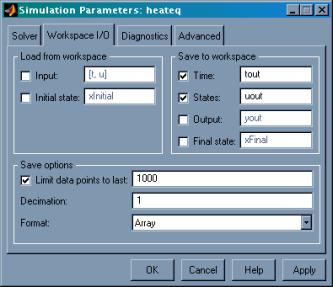
and then plot it with surf. To do this, go to the menu item Simulation Parameters… in
the Simulation menu
of the model. Under the Solver tab, set the stop time to
4.0 (since we are only going out to t
= 4), and under the Workspace I/O tab, check the box to "save states to
Workspace", like this:
After
you run the model, you will find in your Workspace a 53´1 vector tout, plus a 53´9 matrix uout. Each row of these arrays corresponds to a single time step, and
each column of uout corresponds to one value of x.
But remember that we have to add in the values of u at the endpoints as additional columns in u. So we plot the data as follows:
u = [15*ones(length(tout),1), uout, 25*ones(length(tout),1)];
x = -5:5;
surf(x, tout, u)
xlabel('x'), ylabel('t'), zlabel('u')
title('solution to heat equation in a rod')
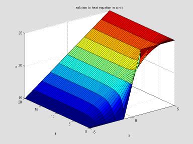
Note how similar this is to the picture obtained before. We leave it to the reader to modify the model for the case of variable heat conductivity.
Solution with pdepe
A
new feature of MATLAB 6.0 is a built-in solver for partial differential
equations in one space dimension (as well as time t). To find out more about
it, read the online help on pdepe. The instructions for use of pdepe are quite explicit but somewhat complicated. The method it uses is somewhat similar to that used in the
SIMULINK solution above; i.e., it uses an ODE solver in t and finite differences in x. The following M-file solves the second
problem above, the one with variable conductivity:
function
heateqex2
%Solves
a sample Dirichlet problem for the heat equation in a rod,
%this
time with variable conductivity, 21 mesh points
m
= 0; %This simply means geometry is
linear.
x
= linspace(-5,5,21);
t
= linspace(0,4,81);
sol
= pdepe(m,@pdex,@pdexic,@pdexbc,x,t);
%
Extract the first solution component as u.
u
= sol(:,:,1);
%
A surface plot is often a good way to study a solution.
surf(x,t,u)
title('Numerical
solution computed with 21 mesh points in x.')
xlabel('x'),
ylabel('t'), zlabel('u')
%
A solution profile can also be illuminating.
figure
plot(x,u(end,:))
title('Solution
at t = 4')
xlabel('x'),
ylabel('u(x,4)')
%
--------------------------------------------------------------
function
[c,f,s] = pdex(x,t,u,DuDx)
c
= 1;
f
= (1 + (x/5).^2)*DuDx;% flux is variable conductivity times u_x
s
= 0;
%
--------------------------------------------------------------
function
u0 = pdexic(x)
%
initial condition at t = 0
u0
= 20+5*sign(x);
%
--------------------------------------------------------------
function
[pl,ql,pr,qr] = pdexbc(xl,ul,xr,ur,t)
%
q's are zero since we have Dirichlet conditions
%
pl = 0 at the left, pr = 0 at the right endpoint
pl
= ul-15;
ql
= 0;
pr
= ur-25;
qr
= 0;
Running
it gives:
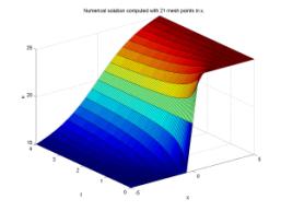
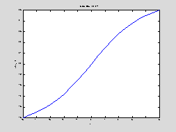
Again the results are very similar to those obtained before.