A Model of Traffic Flow
Everyone has had the experience of
sitting in a traffic jam, or of seeing cars bunch up on a road for no apparent
good reason. MATLAB and SIMULINK are
good tools for studying models of such behavior. Our analysis here will be based on so-called
"follow-the-leader" theories of traffic flow, about which you can
read more in Kinetic Theory of Vehicular
Traffic, by Ilya Prigogine and Robert Herman, Elsevier, New York, 1971, or
in The Theory of Road Traffic Flow,
by Winifred Ashton, Methuen, London, 1966.
We will analyze here an extremely simple model that already exhibits
quite complicated behavior. We consider
a one-lane, one-way, circular road with a number of cars on it (a very
primitive model of, say, the Inner Loop of the Capital Beltway around
Washington, DC, since in very dense traffic, it is hard to change lanes and
each lane behaves like a one-lane road).
Each driver slows down or speeds up on the basis of his own speed, the
speed of the car ahead of him, and the distance to the car ahead of him. But human drivers have a finite reaction time. In other words, it takes them a certain amount of time (usually
about a second) to observe what is going on around them and to press the gas
pedal or the brake, as appropriate. The
standard "follow-the-leader" theory supposes that
![]() ,
(*)
,
(*)
where
t is time, T is the reaction time, un
is the position of the nth car, and
the "sensitivity coefficient" l may depend on ![]() , the spacing between cars, and/or
, the spacing between cars, and/or ![]() , the speed of the nth
car. The idea behind this equation is
this. A driver will tend to decelerate
if he is going faster than the car in front of him, or if he is close to the
car in front of him, and will tend to accelerate if he is going slower than the
car in front of him. In addition, a
driver (especially in light traffic) may tend to speed up or slow down
depending on whether he is going slower or faster (respectively) than a
"reasonable" speed for the road (often, but not always, equal to the
posted speed limit). Since our road is
circular, in this equation u0
is interpreted as uN,
where N is the total number of cars.
, the speed of the nth
car. The idea behind this equation is
this. A driver will tend to decelerate
if he is going faster than the car in front of him, or if he is close to the
car in front of him, and will tend to accelerate if he is going slower than the
car in front of him. In addition, a
driver (especially in light traffic) may tend to speed up or slow down
depending on whether he is going slower or faster (respectively) than a
"reasonable" speed for the road (often, but not always, equal to the
posted speed limit). Since our road is
circular, in this equation u0
is interpreted as uN,
where N is the total number of cars.
The simplest version of the model is the
one where the "sensitivity coefficient" l is a (positive) constant. Then we have a homogeneous linear
differential/difference equation with constant coefficients for the velocities ![]() . Obviously there is
a "steady state" solution when all the velocities are equal and
constant (i.e., traffic is flowing at a uniform speed), but what we are
interested in is the stability of the flow, or the question of what effect is
produced by small differences in the velocities of the cars. The solution of (*) will be a superposition of exponential
solutions of the form
. Obviously there is
a "steady state" solution when all the velocities are equal and
constant (i.e., traffic is flowing at a uniform speed), but what we are
interested in is the stability of the flow, or the question of what effect is
produced by small differences in the velocities of the cars. The solution of (*) will be a superposition of exponential
solutions of the form ![]() = exp(a t)
vn, where the v's and a are (complex) constants,
and the system will be unstable if the velocities are unbounded, i.e., there
are any solutions where the real part of a is positive. Using vector notation, we have
= exp(a t)
vn, where the v's and a are (complex) constants,
and the system will be unstable if the velocities are unbounded, i.e., there
are any solutions where the real part of a is positive. Using vector notation, we have
![]() = exp(a t) v,
= exp(a t) v, ![]() = a exp(a T) exp(a t) v.
= a exp(a T) exp(a t) v.
Substituting
back in (*), we get the equation
a exp(a T) exp(a t) v = l ( S
- I )
exp(a t)
v,
where
S = 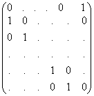
is
the "shift" matrix that, when it multiplies a vector on the left,
cyclically permutes the entries of the vector.
We can cancel the exp(a t) on each side to get
a exp(a T) v = l ( S
- I )
v,
or ( S - (1 + ((a / l) exp(a T)
)I ) v = 0, (**)
which
says that v is an eigenvector for S with eigenvalue![]() . Since the
eigenvalues of S are the Nth roots of unity, which are evenly
spaced around the unit circle in the complex plane, and closely spaced together
for large N, there is potential
instability whenever
. Since the
eigenvalues of S are the Nth roots of unity, which are evenly
spaced around the unit circle in the complex plane, and closely spaced together
for large N, there is potential
instability whenever ![]() has absolute value 1 for some a with positive real part;
that is, whenever
has absolute value 1 for some a with positive real part;
that is, whenever ![]() can be of the form eiq - 1 for some a T
with positive real part. Whether
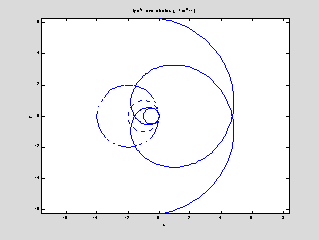
instability occurs or not depends on the value of the product l T. We can see this by plotting values of z exp(z) for z = a T
= i y a complex number on the
critical line Re z = 0, and comparing
with plots of l T (
eiq - 1 ) for various values of
the parameter
can be of the form eiq - 1 for some a T
with positive real part. Whether
instability occurs or not depends on the value of the product l T. We can see this by plotting values of z exp(z) for z = a T
= i y a complex number on the
critical line Re z = 0, and comparing
with plots of l T (
eiq - 1 ) for various values of
the parameter
l T.
syms y;
expand(i*y*(cos(y) + i*sin(y)))
i*y*cos(y)-y*sin(y)
ezplot(-y*sin(y),
y*cos(y), [-2*pi, 2*pi]); hold on
theta = 0:0.05*pi:2*pi;
plot((1/2)*(cos(theta) - 1), (1/2)*sin(theta), '-');
plot(cos(theta) - 1, sin(theta), ':')
plot(2*(cos(theta) - 1), 2*sin(theta), '--');
title('iye^{iy} and circles \lambda T(e^{i\theta}-1)'); hold off
Here
the small solid circle corresponds to lT =
½, and we are just at the limit of stability, since this circle does not cross
the spiral produced by z exp(z) for z a complex number on the critical line Re z = 0, though it "hugs" the spiral closely. The dotted and dashed circles, corresponding
to lT = 1 or 2, do cross the spiral, so they correspond
to unstable traffic flow.
We can check these theoretical predictions
with a simulation using SIMULINK. We'll
give a picture of the SIMULINK model and then explain it.

Here
the Subsystem, which corresponds to multiplication by S - I, looks like this:
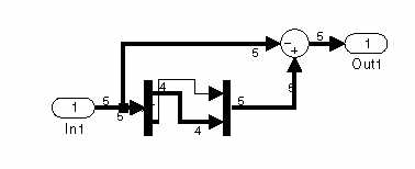
Here are some words of explanation. First of all, we are showing the model using
the options Wide nonscalar lines and Signal dimensions in the Format menu of the SIMULINK model, in
order to show which quantities are vectors and which are scalars. The dimension 5 on most of the lines is the
value of N, the number of cars. Most of the model is like the example in
Chapter 8, except that our unknown function (called u), representing the car positions, is vector-valued and not
scalar-valued. The major exceptions are
these:
1)
We
need to incorporate the reaction-time delay, so we've inserted a Transport
Delay block from the Continuous
block library.
2)
The
parameter l shows up as the value of
the gain in the "sensitivity parameter" Gain block in the upper
right.
3)
Plotting
car positions by themselves is not terribly useful, since only the relative
positions matter. So before outputting
the car positions to the Scope block labeled "relative car
positions," we've subtracted off a constant linear function (corresponding
to uniform motion at the average car speed) created by the Ramp block from the Sources block library.
4)
We've
made use of the option in the Integrator blocks to input the initial
conditions, instead of having them built into the block. This makes the logical structure a little
clearer.
5)
We've
used the subsystem feature of
SIMULINK. If you enclose a bunch of
blocks with the mouse and then click on "Create subsystem" in the
model's Edit menu, SIMULINK will
package them as a subsystem. This is
helpful if your model is large or if there is some combination of blocks that
you expect to use more than once. Our
subsystem sends a vector v to ( S - I ) v = S v - v. A Sum block (with one of the signs changed
to a -) is used for vector subtraction. To model the action of S, we’ve used the
Demux and Mux blocks from the Signals
and Systems block library. The
Demux block, with "number of outputs" parameter set to [4, 1], splits
a 5-dimensional vector into a pair consisting of a 4-dimensional vector and a
scalar (corresponding to the last car).
Then we reverse the order of these and put them back together with the
Mux block, with "number of inputs" parameter set to [1, 4].
Once
the model is assembled, it can be run with various inputs. The following pictures show the two scope
windows with a set of conditions corresponding to stable flow (though, to be
honest, we've let two cars cross through each other briefly!):
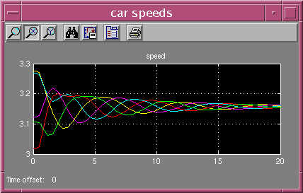
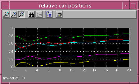
As
you can see, the speeds fluctuate but eventually converge to a single value,
and the separations between cars eventually stabilize.
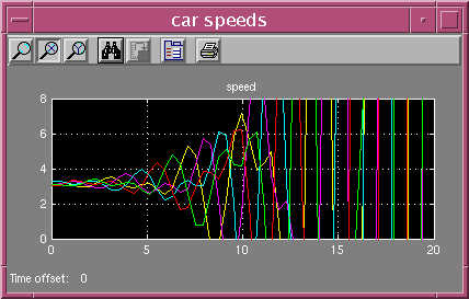
On the other hand, if l is increased by changing
the "sensitivity parameter" in the Gain block in the upper right, say
from 0.8 to 2.0, one gets this sort of output, typical of instability:
We encourage you to go back and tinker with the
model (for instance using a sensitivity parameter that is also inversely
proportional to the spacing between cars) and study the results. We should mention that the To Workspace
block in the lower right has been put in to make it possible to create a movie
of the moving cars. This block sends
the car positions to a variable called carpositions. This variable is what is called a structure array. To make
use of it, you can create a movie with the following script M-file:
theta = 0:0.025*pi:2*pi;
for j = 1:length(tout)
plot(cos(carpositions.signals.values(j,
:)*2*pi), ...
sin(carpositions.signals.values(j,
:)*2*pi), 'o');
axis([-1, 1, -1, 1]);
hold on; plot(cos(theta), sin(theta),
'r'); hold off;
axis equal;
M(j) = getframe;
end
The idea here is that we have taken the circular
road to have radius 1 (in suitable units), so that the command plot(cos(theta),sin(theta),'r') draws a red circle (representing the road) in each
frame of the movie, and on top of that the cars are shown with moving little
circles. The vector tout is a
list of all the
values of t at which the model
computes the values of the vector u(t), and at the jth time, the car positions are stored in the jth row of the matrix carpositions.signals.values. Try the program!
We should mention here one fine point needed to
create a realistic movie. Namely, we
need the values of tout to be equally spaced —
otherwise the cars will appear to be moving faster when the time steps are
large, and will appear to be moving slower when the time steps are small. In its default
mode of operation, SIMULINK uses a variable-step differential equation solver
based on MATLAB's command ode45, so the entries of tout will not be equally
spaced. To fix this, open the Simulation Parameters dialog box using
the Edit menu in the model window, choose the Solvers tab, and change the Output options box to read: Produce
specified output only, chosen to be something like [0:0.5:20]. Then the model will output the car positions only at multiples of
t = 0.5, and the MATLAB program above
will produce a 41-frame movie.
