This book is our attempt to enrich and enliven the teaching of multivariable calculus and mathematical methods courses for scientists and engineers. Most books in these subjects are not substantially different from those of fifty years ago. (Well, they may include fancier graphics and omit several topics, but those are minor changes.) This book is different. We do touch on most of the classical topics; however, we have made a particular effort to illustrate each point with a significant example. More importantly, we have tried to bring fundamental physical applications - Kepler's laws, electromagnetism, fluid flow, energy estimation - back to a prominent position in the subject. From one perspective, the subject of multivariable calculus only exists because it can be applied to important problems in science.
In addition, we have included a discussion of the geometric invariants of curves and surfaces, providing, in effect, a brief introduction to differential geometry. This material provides a natural extension to the traditional syllabus.
We believe that we have succeeded (in resurrecting material that used to be in the course while introducing new material) for one simple reason: we use the computational power of the mathematical software system Mathematica to carry a large share of the load. Mathematica is tightly integrated into every portion of this book. We use its graphical capabilities to draw pictures of curves and surfaces; we use its symbolical capabilities to compute curvature and torsion; we use its numerical capabilities to tackle problems that are well beyond the typical mundane examples of textbooks that treat the subject without using a computer. As an added convenience for the user, we have included with this book a computer disk, where the Mathematica programs used in the text are reproduced.
As an additional benefit from introducing Mathematica, we are able to improve students' understanding of important elements of the traditional syllabus. Our students are better able to visualize regions in the plane and in space. They develop a better feel for the geometric meaning of the gradient; for the method of steepest descent; for the orthogonality of level curves and gradient flows. Because they have tools for visualizing cross sections of solids, they are better able to find the limits of integration in multiple integrals.
To summarize, we think this book is special because, by using it:
We thank several of our colleagues who helped test preliminary
versions of this book in their classrooms: Der-Chen Chang, Paul Green,
Oscar Gonzalez, Alessandra Iozzi, Jonathan Poritz, and Garrett Stuck.
We also thank
Alvaro Alvarez-Parrilla and Nic Ormes, who served capably as teaching
assistants. Finally, we thank four TELOS reviewers for their very helpful
comments on the manuscript: William Barker of Bowdoin
College, Al Hibbard of Center College, Iowa,
Jamie Radcliffe of the University of Nebraska--Lincoln, and Todd Young,
formerly at Northwestern University and now at Ohio University.
We have tried to modernize the course, in part by introducing the mathematical software system Mathematica as a powerful tool. Here are our reasons:
Second, most of the numbers, formulas, and equations found in standard problems are highly contrived to make the computations tractable. This places an enormous limitation on the faculty member trying to present meaningful applications, and lends an air of untruthfulness to the course. (Think about the limited number of examples for an arclength integral that can be integrated easily in closed form.) With the introduction of Mathematica, this drawback is ameliorated. The numerical and symbolic power of Mathematica greatly expands our ability to present realistic examples and applications.
Third, the instructor can concentrate on nonrote aspects of the course. The student can rely on Mathematica to carry out the mundane algebra and calculus that often absorbed all of the student's attention previously. The instructor can focus on theory and problems that emphasize analysis, interpretation, and creative skills. Students can do more than crank out numbers and pictures; they can learn to explain coherently what they mean. This capability is enhanced by the Mathematica Notebook interface, which allows the student to integrate Mathematica commands with output, graphics, and textual commentary.
Fourth, the instructor has time to introduce modern, meaningful subject matter into the course. Because we can rely on Mathematica to carry out the computations, we are free to emphasize the ideas. In this book, we concentrate on aspects of geometry and physics that are truly germane to the study of multivariable calculus. With the introduction of Mathematica, this material can, for the first time, be presented effectively at the sophomore level.
Each chapter is accompanied by a problem set. The problem sets constitute an integral part of the book. Solving the problems will expose you to the geometric, symbolic, and numerical features of multivariable calculus. Many of the problems (especially in Problem Sets C-I) are not routine.
Each problem set concludes with a Glossary of Mathematica commands, accompanied by a brief description, which are likely to be useful in solving the problems in that set. A more complete Glossary, with examples of how to use the commands, is included at the back of the book. In addition, the book contains Mathematica Tips, Sample Notebook Solutions, and an Index. Finally, the accompanying disk contains:
Chapter 1, Introduction, and Problem Set A, Review of One-Variable Calculus, describe the purpose of the book and its prerequisites. The Problem Set reviews both the elementary Mathematica commands and the fundamental concepts of one-variable calculus needed to use Mathematica to study multivariable calculus.
Chapter 2 and Problem Set B, on Vectors and Graphics, introduce the mathematical idea of vectors in the plane and in space. We explain how to work with vectors in Mathematica and how to graph curves and surfaces in space.
Chapter 3, Geometry of Curves, and Problem Set C, Curves, examine parametric curves, with an emphasis on geometric invariants like speed, curvature, and torsion, which can be used to study and characterize the nature of different curves.
Chapter 4, Kinematics, and Problem Set D, Kinematics, apply the theory of curves to the physical problems of moving particles and planets.
Chapter 5, Directional Derivatives, and Problem Set E, Directional Derivatives and the Gradient, introduce the differential calculus of functions of several variables, including partial derivatives, directional derivatives, and gradients. We also explain how to graph functions and their level curves or surfaces with Mathematica.
Chapter 6, Geometry of Surfaces, and Problem Set F, Surfaces, study parametric surfaces, with an emphasis on geometric invariants, including several forms of curvature, which can be used to characterize the nature of different surfaces.
Chapter 7, Optimization in Several Variables, and Problem Set G, Optimization, discuss how calculus can be used to develop numerical algorithms. We also explain how to use Mathematica to test and apply these algorithms in concrete problems.
Chapter 8 and Problem Set H, on Multiple Integrals, develop the integral calculus of functions of several variables. We show how to use Mathematica to set up multiple integrals, as well as how to evaluate them.
Chapter 9, Physical Applications of Vector Calculus, and Problem Set I, Physical Applications, develop the theories of gravitation, electromagnetism, and fluid flow, and then use them with Mathematica to solve concrete problems of practical interest.
Chapter 10, Mathematica Tips, gathers together the answers to many Mathematica questions that have puzzled our students. Read through this chapter at various times as you work through the rest of the book. If necessary, refer back to it when some aspect of Mathematica has you stumped.
The Glossary includes all the commands from the Problem Set glossaries - together with illustrative examples - plus some additional entries.
The Sample Notebook Solutions contain sample solutions to one or more problems from each Problem Set. These samples can serve as models when you are working out your own solutions to other problems.
Finally, we have a comprehensive Index of Mathematica commands and mathematical concepts that are found in this book.
We assume that you know how to start Mathematica on your computer. We also assume that you are familiar with elementary Mathematica commands to do arithmetic, algebra, and one-variable calculus. More precisely, we assume that you can Factor and Simplify algebraic expressions, Solve equations, and differentiate, integrate, and compute limits (with the Mathematica commands D, Integrate, and Limit). Finally, we assume that you can Plot functions of one variable. Problem Set A tests exactly this body of knowledge in Mathematica.
We also assume that you can use Mathematica Notebooks - in particular, that you can combine input, output, graphics, and text to produce a coherent and attractive document. You can learn how to use Mathematica Notebooks from any of the primers cited below. You may also consult The Mathematica Book, Third Edition, by Stephen Wolfram (Wolfram Media, Inc. and Cambridge University Press, 1996), but that is a reference book of far greater scope than is required here.
If necessary, you can quickly gain expertise in Mathematica from the online help online Help Browser or from one of the following primers:
More Mathematica books are being published all the time. You can find an up-to-date list in the bookstore section of the Wolfram Research web site.
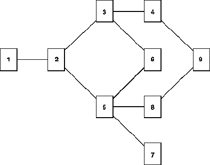
If, as in our courses, this book supplements a traditional text, then it contains more material than can be covered in a single semester. To aid in selecting a coherent subset of the material, here is a diagram showing the dependence among the chapters:
We suggest that you work all the problems in Problem Set A, read Chapter 2, and then work at least a quarter to a half of Problem Set B. After that, various combinations of chapters are possible. Here are a few selections that we have found suitable for a one-semester multivariable calculus course:
In a problem seminar or mathematical methods course, more flexibility is possible, and we could choose a greater variety of problems from various chapters.
Beginning with Problem Set C, the exercises in the Problem Sets become fairly substantial; it is easy to spend an hour on each problem. To ease the burden, we often allow students to collaborate on the problems in groups of two or three. We ask each collaborating team to turn in a single joint assignment. This system fosters teamwork, builds confidence, and makes the harder problems manageable.
The problems in this book have been classroom-tested according to two different schemes. Problems can be assigned in big chunks, as projects to be worked on three or four times during the term. Alternatively, problems can be assigned one or two at a time on a more regular basis. Both methods work; which works better depends on the backgrounds of instructor and students, and on how thoroughly you want to combine the material from this book with assignments from a standard textbook.